Preprocess¶

This manual shows an example of the preprocessing pipeline using the interactive calibration module of 'prepGUI'. To run the preprocessing module, you should first check the data and their path.

The 'raw' and 'cal' directories should be in the base directory. In the 'raw' directory, object frames should be stored in each target directory such as 'ARxxxxxx'. In addition to the object frames, biasdark frames should also exist because these biasdark frames have information about the setting of each run of observation. To correctly calibrate these object frames, you should check whether at least one biasdark frame and flat frame exist in the 'cal' directory. If the preprocessing code is operated properly, the outcome 'proc' and 'comp' directories will be made in the base directory. Each fringe frame and master flat frame will be stored in the './proc/cal' directory, and the calibrated object frame will be saved in the target directory. Below is an example directory tree.

basedir
└───raw
│   └───ARxxxxxx
│       │   FISS_YYYYMMDD_hhmmss.zzz_A.fts
│       │   FISS_YYYYMMDD_hhmmss.zzz_A_BiasDark.fts
│       │   ...
└───cal
│   │   FISS_YYYYMMDD_hhmmss.zzz_A_Flat.fts
│   │   FISS_YYYYMMDD_hhmmss.zzz_A_BiasDark.fts
│   │   ...
└───proc
│   └───ARxxxxxx
│       │   FISS_YYYYMMDD_hhmmss.zzz_A1.fts
│       │   ...
│   └───cal
│       │   FISS_FLAT_YYYYMMDD_hhmmss.zzz_A.fts
│       │   FISS_FLAT_YYYYMMDD_hhmmss.zzz_A.fts
│       │   FISS_xFringe_YYYYMMDD_hhmmss.zzz_A.fts
│       │   FISS_yFringe_YYYYMMDD_hhmmss.zzz_A.fts
│       │   ...
└───comp
    └───ARxxxxxx
        │   FISS_YYYYMMDD_hhmmss.zzz_A1_c.fts
        │   ...

If you prepare the data, you also check the authority of the directory and data. The raw data should be readable, and the base directory should be able to read and write.

After setting the data, let's run the preprocess GUI using fisspy.process.prepGUI. It automatically sets the matplotlib backend to the Qt5 backend. Please do not run this backend in the jupyter-notebook, but run it in the ipython.

Step 0: Select the flat frame¶

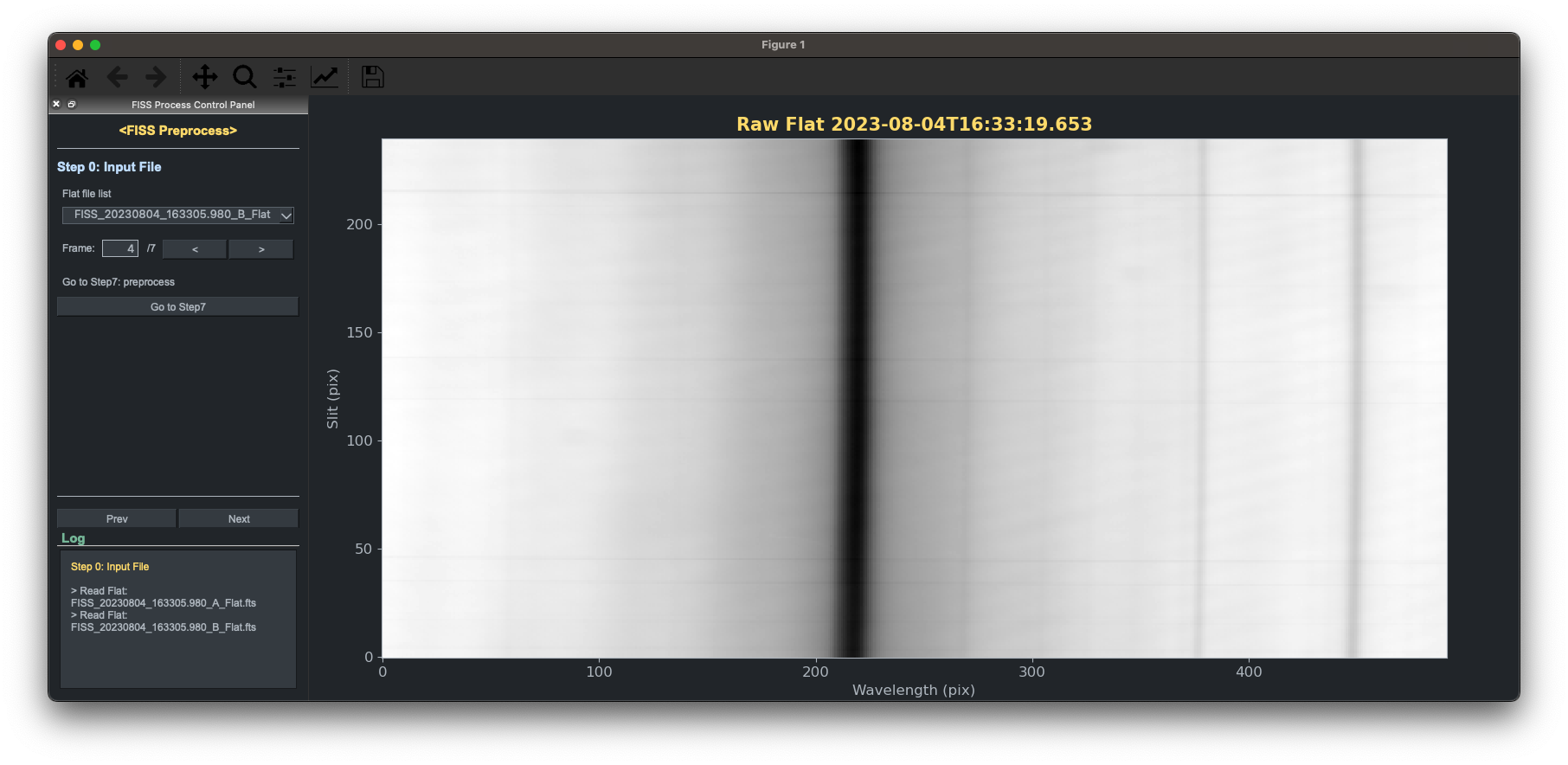
When you run the 'prepGUI' at first, it shows the GUI figure that you can select the flat frame. After setting the flat frame then push the next button to go to the next step.

Step 1: Tilt correction¶

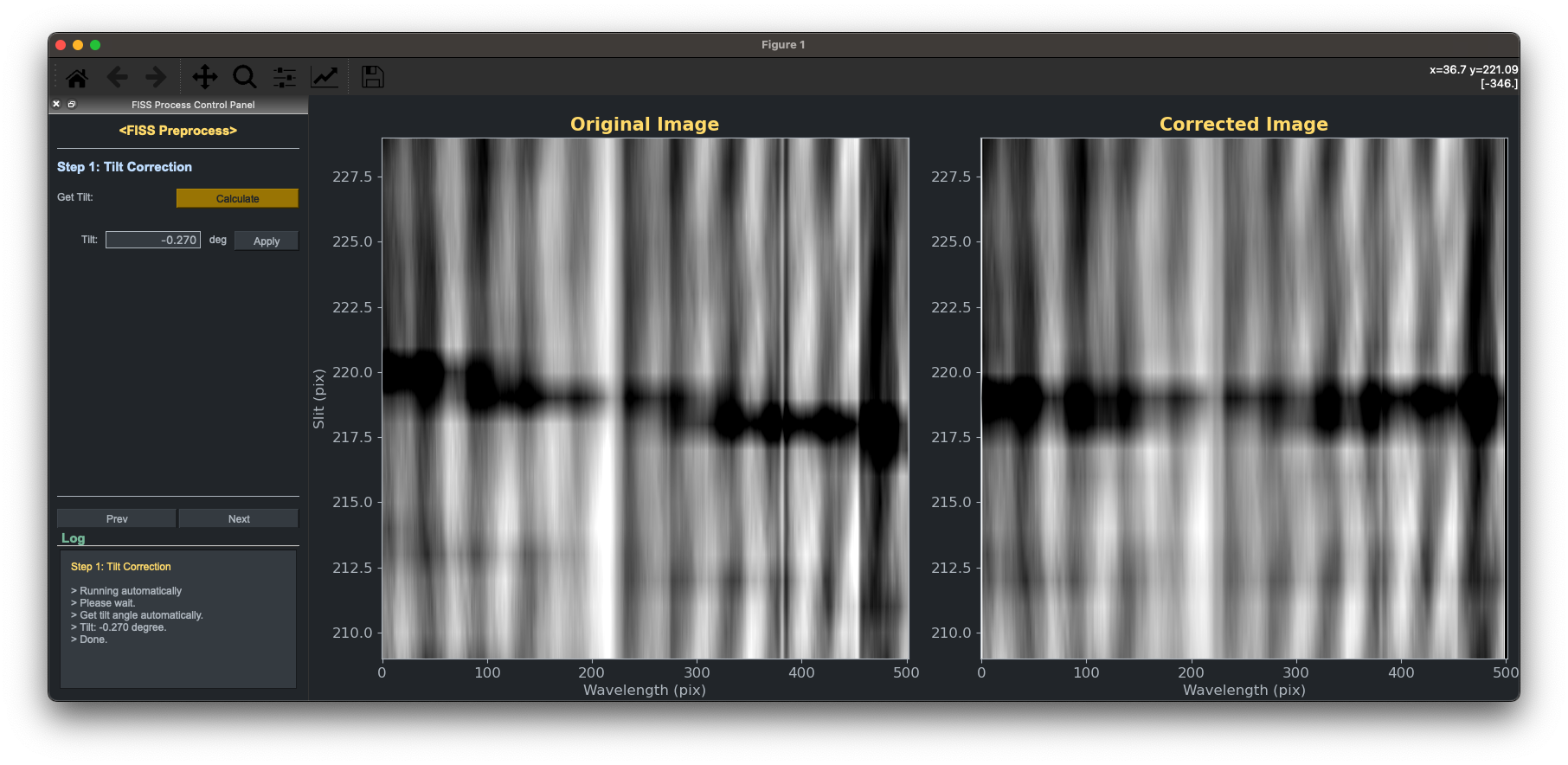
After selecting the flat frame, the first we have to do is the tip/tilt correction of the image. If you put the ffocA and ffocB parameters when you call the 'prepGUI' module, it automatically corrects the tip/tilt using the pinhole focus frame. If not it corrects the tip/tilt using the slit pattern generated by the dust on the slit. Here you can manually change the tip/tilt angle putting the value.

Step 2: 1st Curvature Correction¶

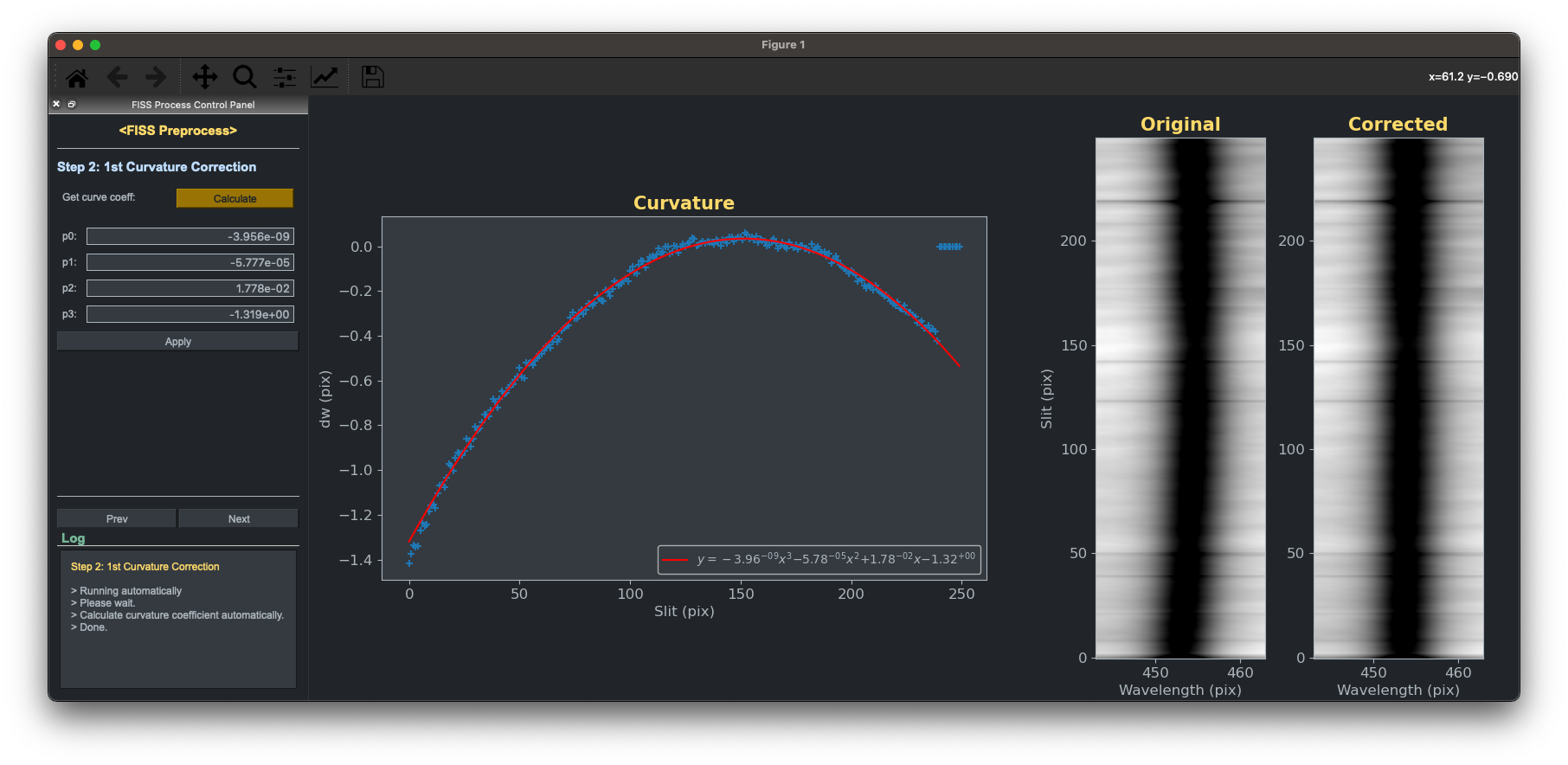
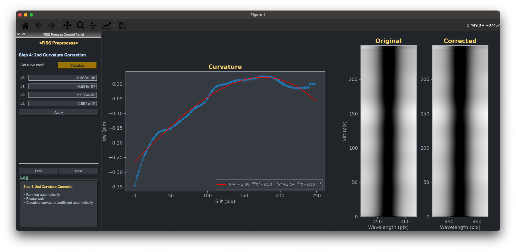
The next step is to correct the distortion or curvature of the frame. You can notice that the spectral line is curved on the raw data. Using the cross-correlation technique, we measure the shift value by pixel-to-pixel, and finally, we correct this curvature by 3rd-order polynomial fitting.

Step 3: Atlas Subtraction¶

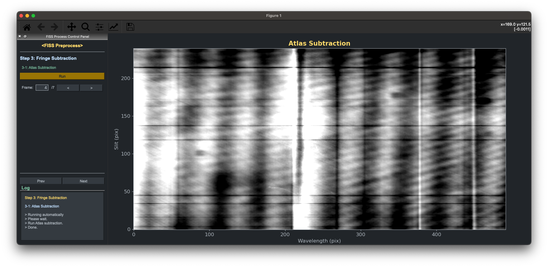
To enhance the fringe pattern on the image frame, we divide the atlas spectrum. As a result, we can easily identify the fringe patterns.

Step 4: Horiziontal fringe subtraction¶

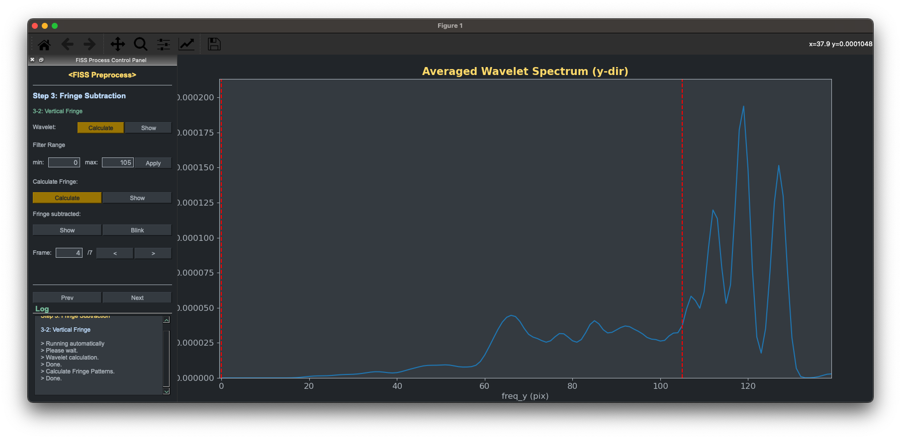
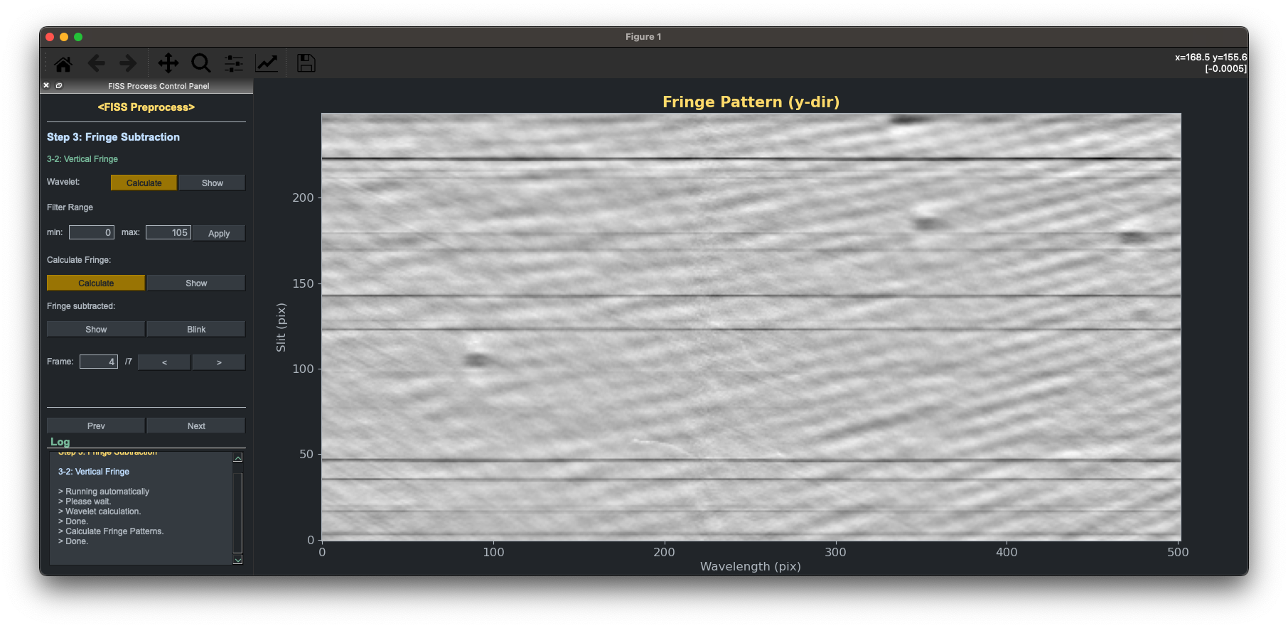
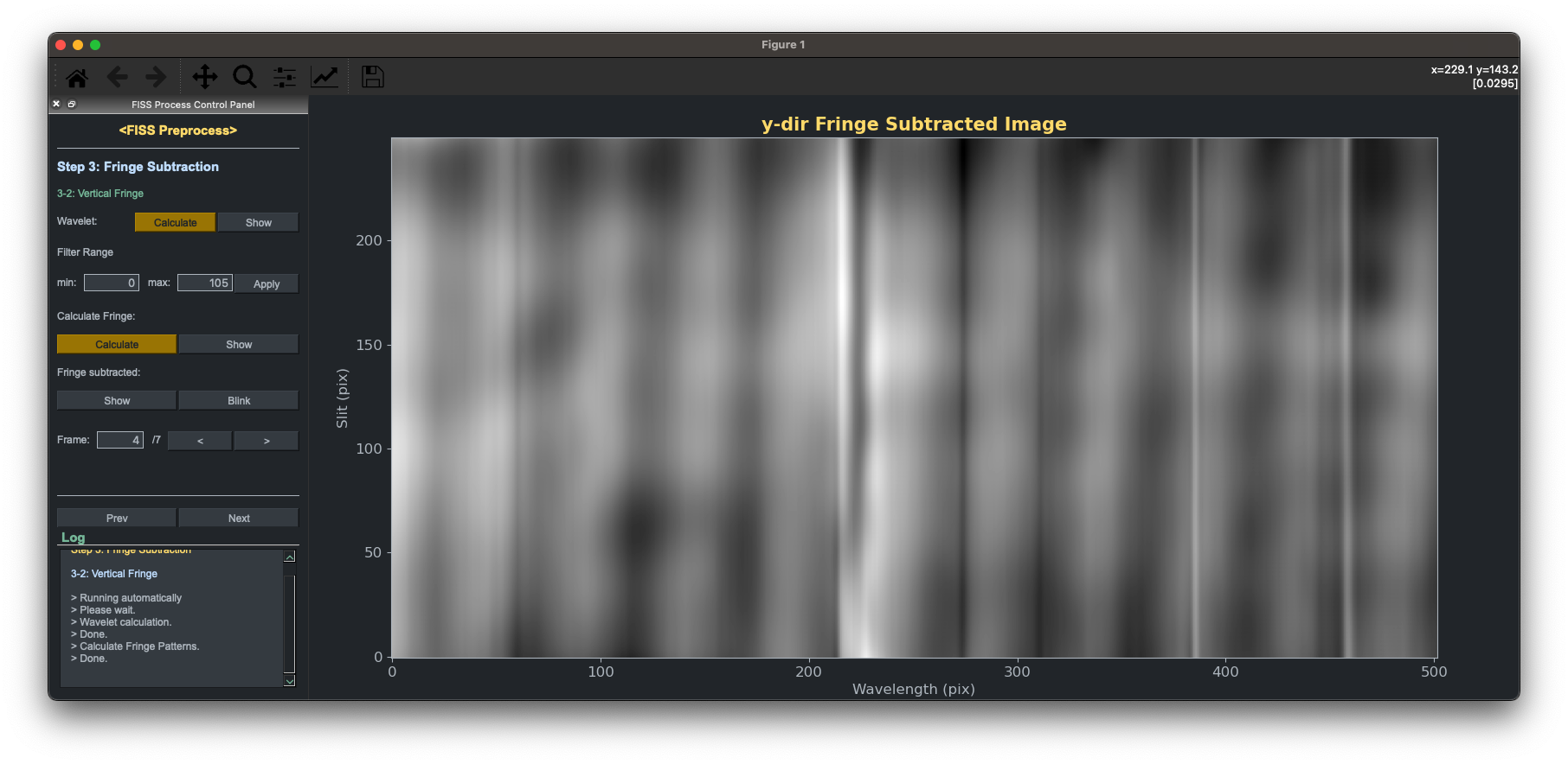
Now we subtract the horizontal fringe first by using the wavelet spectrum. The program automatically runs the wavelet along the y-axis. We empirically set the filtering range that contributes to the fringe pattern from 0 to 105, but we recommend you that change this value if this range covers the actual data that comes from the flat pattern with the peak in the power spectrum. Here, you can see the fringe pattern, and the fringe subtracted pattern by pushing the show button on each panel.

Step 5 (It will be run only for the cam B!): Mask spectra¶

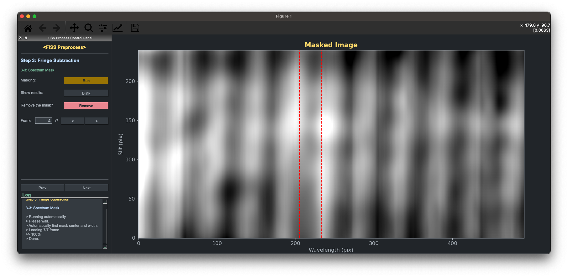
To subtract the vertical fringe only, we should mask the actual spectrum. Here we use the autoregressive interpolation method to fill the masked spectra. It takes some time up to 3 to 5 minutes.

Step 6: Vertical fringe subtraction¶

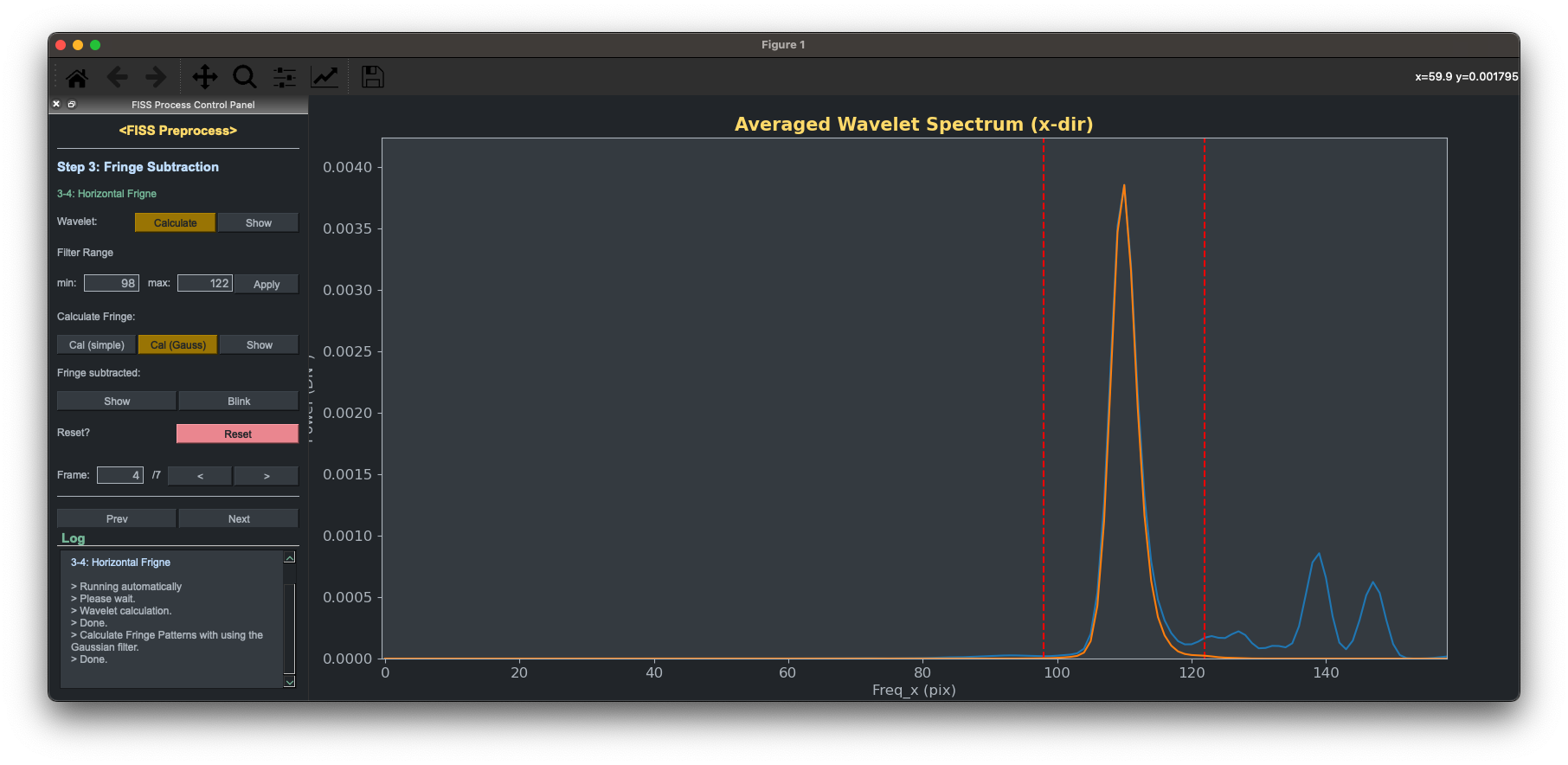
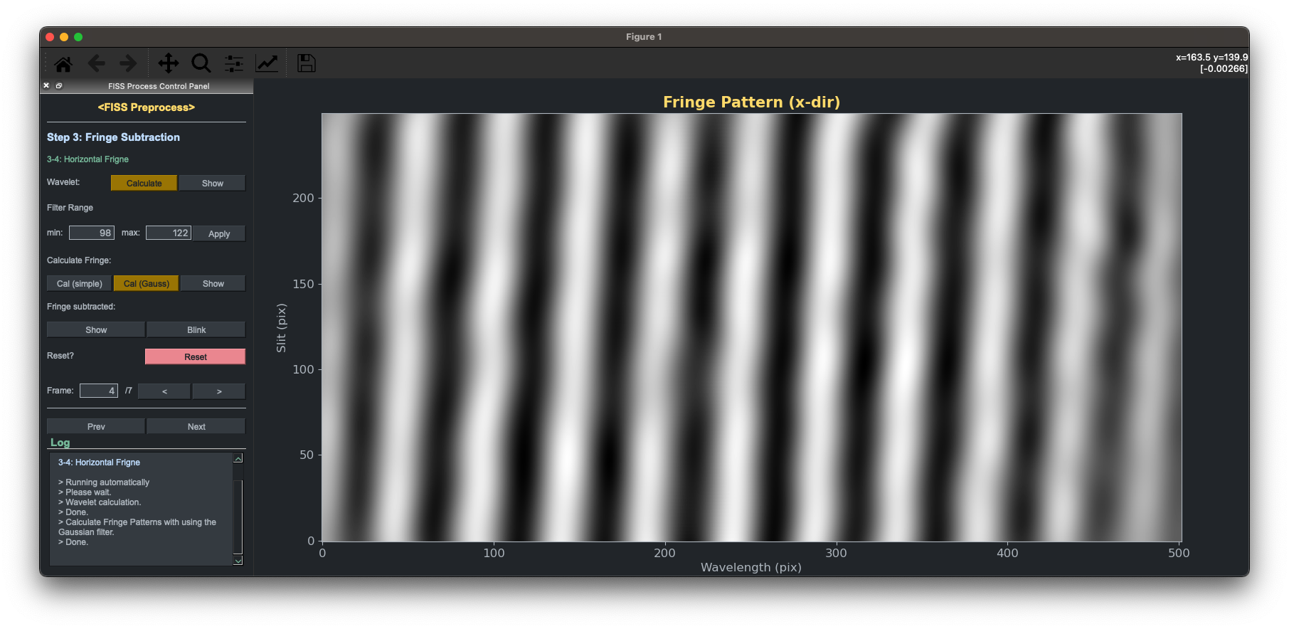
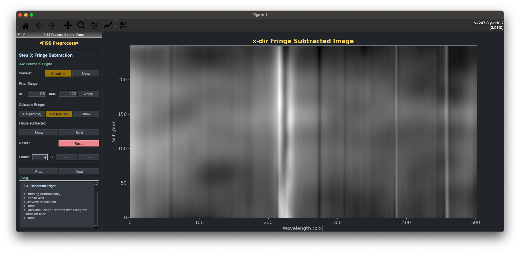
Now we subtract the vertical fringe, select the frequency peak, and apply the Gaussian filter to extract this frequency peak that contributes to the vertical fringe. Similar to step 4, you can check the fringe pattern and fringe subtracted image by pressing the show button on each panel.

Step 7: 2nd curvature correction¶

After subtracting all fringes, we correct the curvature again.

Step 8: Make master flat¶

Now we are ready to run the make a master flat. This procedure is based on Chae et al. (2013). You can see the master flat, the flat corrected image, and the corrected line profile, here.

Step 9: Save data.¶

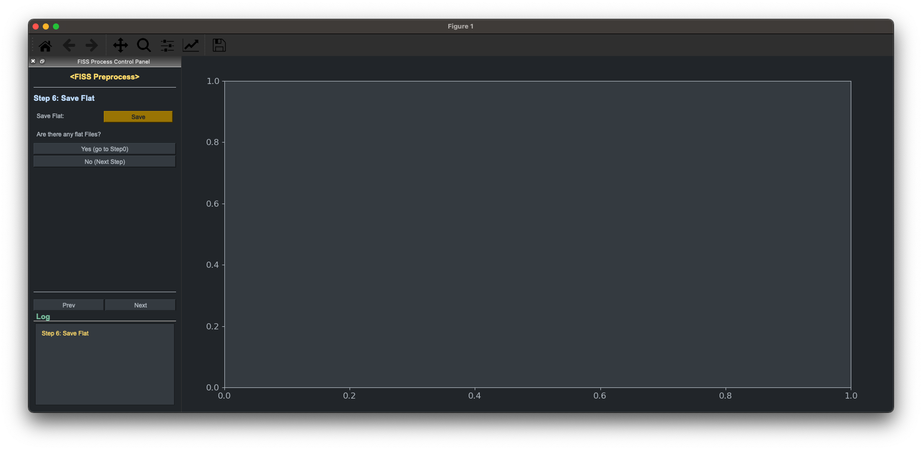
We made the whole calibration. By pushing the save button, you can save these data. There are two options: one is to select the other flat frame to make other calibration data, and the other is to go to the next step. If you already run the calibration for all flat frames, then go to the next step button will be highlighted.

Step 10: Preprocessing

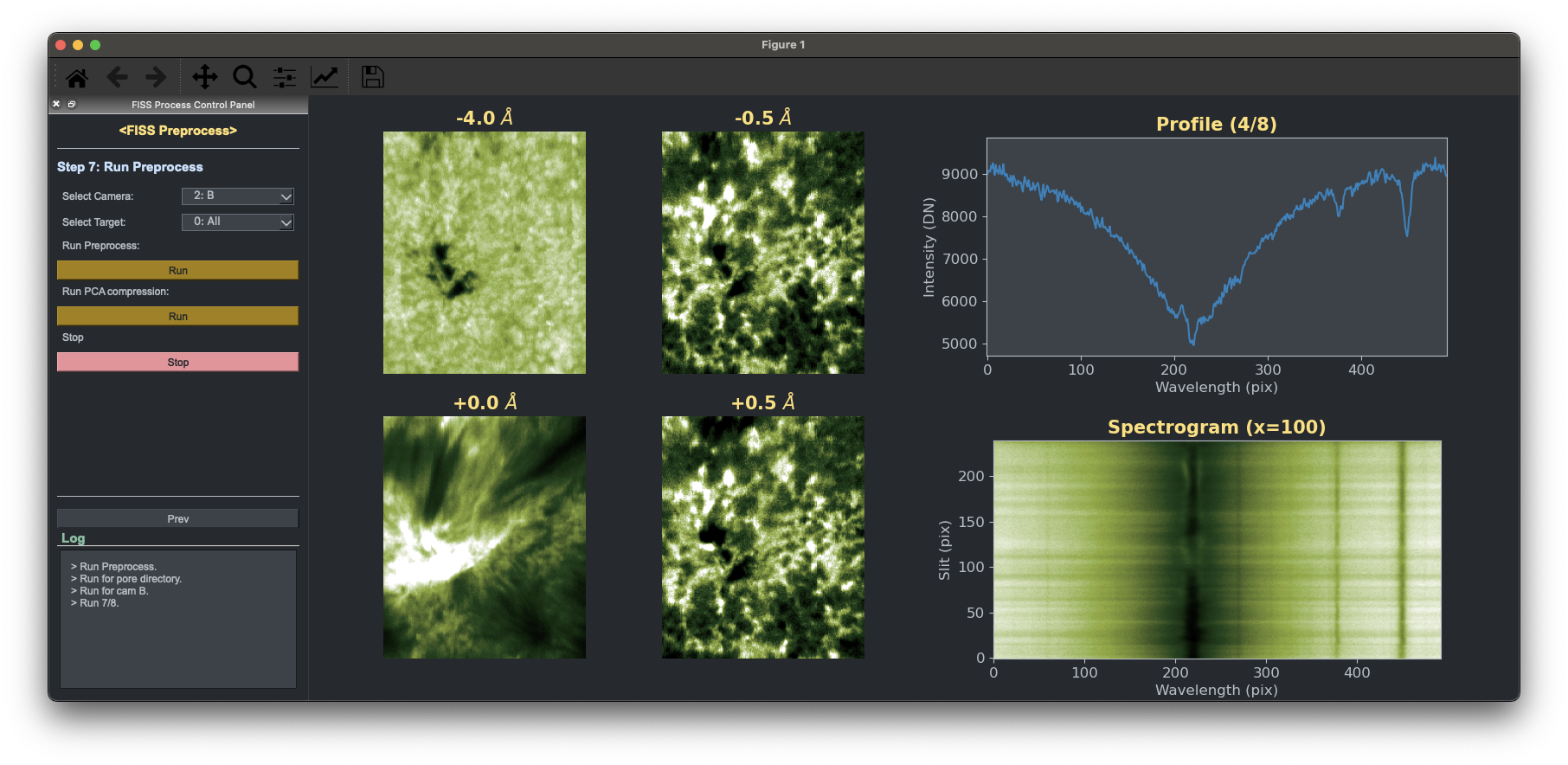
Then let's run the preprocessing pipeline to the object frames. You can run this for the whole data set or separately. Here, If you want to reduce the running time, I recommend you that run this for each data set (I mean for each target or each camera) to reduce the running time by parallelly running this code in the separate terminals.

Step 11: PCA Compression¶

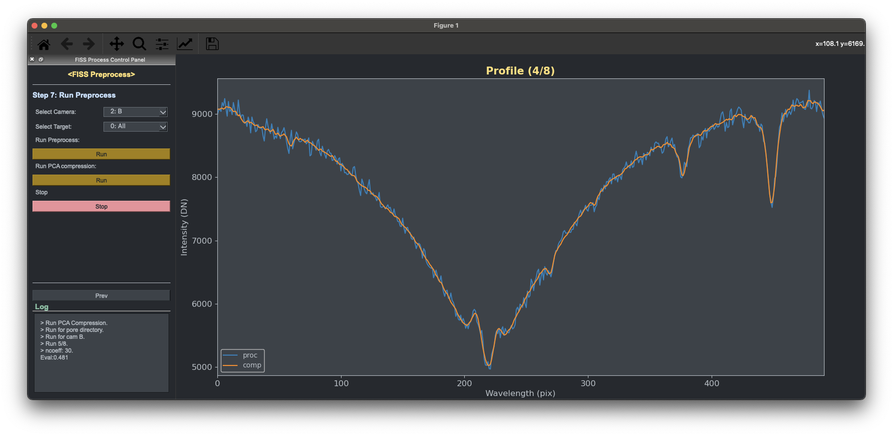
This is the final step of the preprocessing. Now you can compress and denoise the data by using the PCA compression. Just push the run button in the 'Run PCA compression' panel.